Titanic 生存率预测 一、问题描述 泰坦尼克号(Titanic)问题的背景就是那个大家都熟悉的『Jack and Rose』的故事,豪华游艇倒了,大家都惊恐逃生,可是救生艇的数量有限,无法人人都有,副船长发话了『lady and kid first!』,所以是否获救其实并非随机,而是基于一些背景而有rank先后的。训练和测试数据是一些乘客的个人信息以及存活状况,要尝试根据它生成合适的模型并预测其他人(test.data中的新数据)的存活状况,模型最终结果保存在predictedData.csv中。
显然,这是一个二分类问题,我们学习使用集成学习方法进行建模求解。https://www.kaggle.com/competitions/titanic/data
开始加油! (ง •̀_•́)ง (*•̀ㅂ•́)و
1 2 3 4 5 6 7 8 9 10 11 12 13 14 15 16 17 18 19 20 21 22 23 24 25 26 27 28 29 30 31 import numpy as npimport pandas as pdimport seaborn as snsimport matplotlib.pyplot as plt'font.sans-serif' ] = ['SimHei' ] 'axes.unicode_minus' ] = False from sklearn.preprocessing import LabelEncoder from sklearn.model_selection import train_test_split from sklearn.linear_model import LogisticRegressionfrom sklearn.svm import SVC, LinearSVC from sklearn.ensemble import RandomForestClassifierfrom sklearn.neighbors import KNeighborsClassifierfrom sklearn.naive_bayes import GaussianNBfrom sklearn.linear_model import Perceptron from sklearn.linear_model import SGDClassifier from sklearn.tree import DecisionTreeClassifierfrom sklearn.ensemble import GradientBoostingClassifierfrom xgboost import XGBClassifier from lightgbm import LGBMClassifierfrom sklearn.model_selection import GridSearchCV, cross_val_score, StratifiedKFold, learning_curvefrom sklearn.metrics import precision_score import warnings'ignore' )
二、数据读取和查看 首先读入数据,并且初步查看数据的记录数,字段数据类型,缺失等信息。
1 2 3 4 5 'data/train.csv' )'data/test.csv' )
PassengerId
Survived
Pclass
Name
Sex
Age
SibSp
Parch
Ticket
Fare
Cabin
Embarked
0
1
0
3
Braund, Mr. Owen Harris
male
22.0
1
0
A/5 21171
7.2500
NaN
S
1
2
1
1
Cumings, Mrs. John Bradley (Florence Briggs Th...
female
38.0
1
0
PC 17599
71.2833
C85
C
2
3
1
3
Heikkinen, Miss. Laina
female
26.0
0
0
STON/O2. 3101282
7.9250
NaN
S
3
4
1
1
Futrelle, Mrs. Jacques Heath (Lily May Peel)
female
35.0
1
0
113803
53.1000
C123
S
4
5
0
3
Allen, Mr. William Henry
male
35.0
0
0
373450
8.0500
NaN
S
<class 'pandas.core.frame.DataFrame'>
RangeIndex: 891 entries, 0 to 890
Data columns (total 12 columns):
# Column Non-Null Count Dtype
--- ------ -------------- -----
0 PassengerId 891 non-null int64
1 Survived 891 non-null int64
2 Pclass 891 non-null int64
3 Name 891 non-null object
4 Sex 891 non-null object
5 Age 714 non-null float64
6 SibSp 891 non-null int64
7 Parch 891 non-null int64
8 Ticket 891 non-null object
9 Fare 891 non-null float64
10 Cabin 204 non-null object
11 Embarked 889 non-null object
dtypes: float64(2), int64(5), object(5)
memory usage: 83.7+ KB
我们可以看到部分数据存在缺失,数据类型多样,后续需要进行相关的数据处理。
PassengerId
Survived
Pclass
Age
SibSp
Parch
Fare
count
891.000000
891.000000
891.000000
714.000000
891.000000
891.000000
891.000000
mean
446.000000
0.383838
2.308642
29.699118
0.523008
0.381594
32.204208
std
257.353842
0.486592
0.836071
14.526497
1.102743
0.806057
49.693429
min
1.000000
0.000000
1.000000
0.420000
0.000000
0.000000
0.000000
25%
223.500000
0.000000
2.000000
20.125000
0.000000
0.000000
7.910400
50%
446.000000
0.000000
3.000000
28.000000
0.000000
0.000000
14.454200
75%
668.500000
1.000000
3.000000
38.000000
1.000000
0.000000
31.000000
max
891.000000
1.000000
3.000000
80.000000
8.000000
6.000000
512.329200
以上包含数值型数据(Numerical data)的统计特征
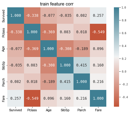
三、数据探索与变量分析 首先通过pandas的corr()函数计算相关系数矩阵,初步探索各个字段与预测变量“Survived”的关系以及各个变量之间的关系。
1 2 3 4 5 6 7 8 9 10 11 12 13 14 'PassengerId' ,axis=1 ).corr()9 ,6 ))'ggplot' )'darkgrid' )set (context="paper" , font="monospace" )20 , 220 , n=200 ),cbar=True , annot=True , square=True , fmt='.3f' ,'size' :12 })11 )11 )'train feature corr' , fontsize=15 )
Text(0.5, 1.0, 'train feature corr')
根据相关系数矩阵,我们初步分析可知:
Fare(乘客费用)、Parch(同行的家长和孩子数目)与“Survived”正相关。
SibSp(同行的兄弟姐妹和配偶数目)、Age(年龄)、Pclass(用户阶级)与
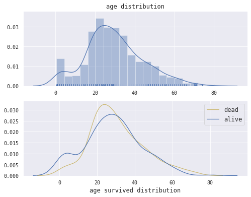
四、特征探索 4.1 年龄(Name) 我们将可视化展示训练数据集中年龄的整体分布以及dead和alive乘客的数量分布统计。并进行对比分析。
1 2 3 4 5 6 7 8 9 10 11 12 13 14 15 16 17 18 from scipy import stats2 ,1 ,figsize=(8 ,6 ))True , color='b' , ax=axes[0 ])0 ]10 )'age distribution' ,fontsize=12 )'' )'' )1 ]0 ].Age.dropna(), hist=False , color='y' , ax=ax1, label='dead' )1 ].Age.dropna(), hist=False , color='b' , ax=ax1, label='alive' )10 )'age survived distribution' ,fontsize=12 )'' )12 )
<matplotlib.legend.Legend at 0x24b9bfaffd0>
乘客的年龄集中在20-40岁,所以主要为青年人和中年人。从age survived distribution表中我们可以发现,小孩获救似乎更容易一些,这个结果也有一定的社会基础,灾难时刻,大多数人可能选择站出来保护妇女和儿童。
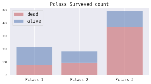
4.2 用户阶级(Pclass) 我们绘制柱形图展示不同Pclass(1, 2 , 3)的乘客获救与未获救的数量,以对比发现Pclass与“Survived”的关系。
1 2 3 4 5 6 7 8 9 10 11 y_dead = train_df[train_df.Survived==0 ].groupby('Pclass' )['Survived' ].count()1 ].groupby('Pclass' )['Survived' ].count()1 ,2 ,3 ]8 ,4 )).add_subplot(1 ,1 ,1 )'r' , alpha=0.5 , label='dead' )'b' , bottom=y_dead, alpha=0.5 , label='alive' )15 , loc='best' )'Pclass %d' %(i) for i in range (1 ,4 )], size=12 )'Pclass Surveved count' , size=15 )
Text(0.5, 1.0, 'Pclass Surveved count')
Pclass从1至3等级递减,即1可以理解为头等乘客。我们发现在Pclass=1的记录中,乘客的获救比例明显最高,这是一个有趣的现象。或许更高等的乘客配备了更好的保护措施。
4.3 性别(Sex) 1 2 3 4 5 print (train_df.Sex.value_counts())print ('-------------------------------' )print (train_df.groupby('Sex' )['Survived' ].mean())
male 577
female 314
Name: Sex, dtype: int64
-------------------------------
Sex
female 0.742038
male 0.188908
Name: Survived, dtype: float64
我们注意到,男性的数量偏多,同时数据展现出来的女性的存活率(0.742038)远远高于男性(0.188908)
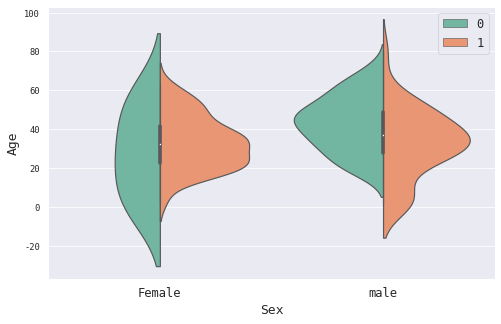
1 2 3 4 5 6 7 8 8 ,5 )).add_subplot(1 ,1 ,1 )'Sex' , y='Age' , hue='Survived' , palette="Set2" , data=train_df.dropna(), split=True )'Sex' , size=13 )'Female' , 'male' ], size=12 )'Age' , size=13 )12 ,loc='best' )
<matplotlib.legend.Legend at 0x24b9e256f40>
图例中0表示’Survived’=0,即未获救;图表具有多个维度,可以反映不同性别以及是否获救的乘客的大致分布情况。
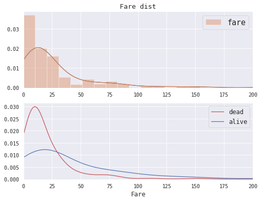
4.4 Frae(票价) 我们分别绘制票价的总体分布图和dead和alive类型的票价分布对比图
1 2 3 4 5 6 7 8 9 10 11 12 13 14 15 16 17 18 19 20 21 22 23 24 25 8 , 6 ))2 ,2 ), (0 ,0 ), colspan=2 )10 )'Fare dist' , size=13 )'fare' , ax=ax)15 )range (0 ,201 ,25 )0 , 200 ])'' )'' )2 ,2 ), (1 ,0 ), colspan=2 )10 )0 ].Fare, ax=ax1,hist=False , label='dead' , color='r' )1 ].Fare, ax=ax1,hist=False , label='alive' , color='b' )0 ,200 ])12 )'Fare' , size=12 )'' )
Text(0, 0.5, '')
图中可以看到,低票价(Fare)的乘客中死亡比例极高,而高票价的乘客中获救的人似乎要更多。
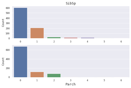
4.5 表亲和直亲(SibSp和Parch) SibSp描述了泰坦尼克号上与乘客同行的兄弟姐妹(Siblings)和配偶(Spouse)数目;
1 2 3 4 5 6 7 8 9 10 11 12 8 , 5 ))2 , 1 , 1 )'SibSp' , size=13 )'' )'Count' ,size=11 )2 , 1 , 2 , sharex=ax1)'Parch' , size=13 )'Count' ,size=11 )
Text(0, 0.5, 'Count')
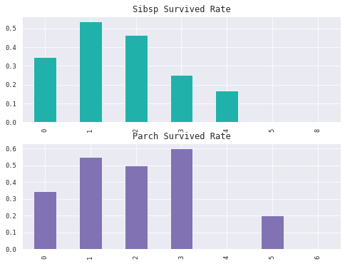
1 2 3 4 5 6 7 8 9 10 11 12 8 ,6 ))2 , 1 , 1 )'SibSp' )['Survived' ].mean().plot(kind='bar' ,ax= ax1,color='lightseagreen' )'Sibsp Survived Rate' , size=12 )'' )2 , 1 , 2 )'Parch' )['Survived' ].mean().plot(kind='bar' ,ax= ax2,color='m' )'Parch Survived Rate' , size=12 )'' )
Text(0.5, 0, '')
分组统计不同亲戚类型,即表亲和直亲(SibSp和Parch)和数量的获救率。我们发现,获救率与亲戚的关系可能并不具有简单的线性关系。
五、特征工程 5.1 Name特征处理 充分挖掘和提取Titanic数据集的特征可以有效提高模型精度。因此,我们对name字段进行挖掘和特征的提取
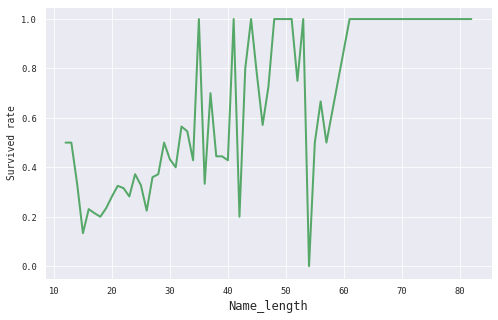
5.2 Name_Len特征 由于西方人的名字长度差别较大,且含义丰富,我们首先探索一下名字长度这个特征:
1 2 3 train_df.groupby(train_df.Name.apply(lambda x: len (x)))['Survived' ].mean().plot(figsize=(8 ,5 ),linewidth=2 ,color='g' )'Name_length' ,fontsize=12 )'Survived rate' )
Text(0, 0.5, 'Survived rate')
可以看到名字的长度和获救率还是有一定的正向关系的,可以考虑加入Name_Len特征:
1 2 3 4 5 'Name_Len' ] = combine_df['Name' ].apply(lambda x: len (x))'Name_Len' ] = pd.qcut(combine_df['Name_Len' ],5 )
注: 数据分箱(也称为离散分箱或分段)是一种数据预处理技术,用于减少次要观察误差的影响,是一种将多个连续值分组为较少数量的“分箱”的方法。
5.3 Title特征 西方人名字中含有的称谓信息(数据集中名字中间的单词)也可以在很大程度上反映一个人的身份地位,从数据中提取”Title”(称谓)也可以作为特征,由于有些称谓的人数量过少,我们还需要做一个映射(分组),将一组等效的称谓合并在一起。
几条有关英语称谓的解释:
Mme: 相当于MrsMs: Ms.或Mz 美国近来用来称呼婚姻状态不明的妇女
Jonkheer: 乡绅Col: 中校:Lieutenant Colonel(Lt. Col.)上校:Colonel(Col.)
Lady: 贵族夫人的称呼Major: 少校
Don唐: 是西班牙语中贵族和有地位者的尊称Mlle: 小姐
sir: 懂的都懂Rev: 牧师
the Countess: 女伯爵测试集合中的Dona :女士尊称
1 2 3 4 5 6 7 8 9 'Title' ] = combine_df['Name' ].apply(lambda x: x.split(', ' )[1 ]).apply(lambda x: x.split('.' )[0 ])'Title' ] = combine_df['Title' ].replace(['Don' ,'Dona' , 'Major' , 'Capt' , 'Jonkheer' , 'Rev' , 'Col' ,'Sir' ,'Dr' ],'Mr' )'Title' ] = combine_df['Title' ].replace(['Mlle' ,'Ms' ], 'Miss' )'Title' ] = combine_df['Title' ].replace(['the Countess' ,'Mme' ,'Lady' ,'Dr' ], 'Mrs' )'Title' ],prefix='Title' )1 )
在特征探索阶段,我们发现男性和女性的获救率分别为女性的0.742038和男性的0.188908;
1 2 3 4 5 6 7 8 9 10 'Surname' ] = combine_df['Name' ].apply(lambda x:x.split(',' )[0 ])list (set (combine_df[(combine_df.Sex=='female' ) & (combine_df.Age>=12 )0 ) & ((combine_df.Parch>0 ) | (combine_df.SibSp > 0 ))]['Surname' ].values))list (set (combine_df[(combine_df.Sex=='male' ) & (combine_df.Age>=12 )1 ) & ((combine_df.Parch>0 ) | (combine_df.SibSp > 0 ))]['Surname' ].values))'Dead_female_family' ] = np.where(combine_df['Surname' ].isin(dead_female_surname),0 ,1 )'Survive_male_family' ] = np.where(combine_df['Surname' ].isin(survive_male_surname),0 ,1 )'Name' ,'Surname' ],axis=1 )
5.4 Age特征 根据特征探索阶段的分析,小孩的获救率明显较高,可以添加一个小孩标签属性(IsChild):
1 2 3 4 5 6 7 'Title' , 'Pclass' ])['Age' ]'Age' ] = group.transform(lambda x: x.fillna(x.median()))'Title' ,axis=1 )'IsChild' ] = np.where(combine_df['Age' ]<=12 ,1 ,0 )'Age' ] = pd.cut(combine_df['Age' ],5 )'Age' ,axis=1 )
5.5 Familysize 将上面提取过的Familysize再离散化
1 2 3 4 5 6 'FamilySize' ] = np.where(combine_df['SibSp' ]+combine_df['Parch' ]==0 , 'Alone' ,'SibSp' ]+combine_df['Parch' ]<=3 , 'Small' , 'Big' ))'FamilySize' ],prefix='FamilySize' )1 ).drop(['SibSp' ,'Parch' ,'FamilySize' ],axis=1 )
5.6 Ticket特征 统计发现,【’1’, ‘2’, ‘P’】开头的Ticket获救率更高。可以标注为’High_Survival_Ticket’型票;同理【’A’,’W’,’3’,’7’】为’Low_Survival_Ticket’型票。这样得到High_Survival_Ticket和Low_Survival_Ticket两个新的特征。
1 2 3 4 5 6 combine_df['Ticket_Lett' ] = combine_df['Ticket' ].apply(lambda x: str (x)[0 ])'Ticket_Lett' ] = combine_df['Ticket_Lett' ].apply(lambda x: str (x))'High_Survival_Ticket' ] = np.where(combine_df['Ticket_Lett' ].isin(['1' , '2' , 'P' ]),1 ,0 )'Low_Survival_Ticket' ] = np.where(combine_df['Ticket_Lett' ].isin(['A' ,'W' ,'3' ,'7' ]),1 ,0 )'Ticket' ,'Ticket_Lett' ],axis=1 )
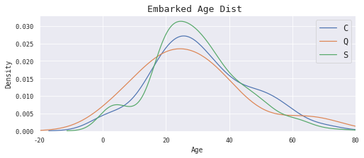
5.7 Embarked特征 1 2 3 4 5 6 7 ax = plt.figure(figsize=(8 ,3 )).add_subplot(111 )20 , 80 ])'C' ].Age.dropna(), ax=ax, label='C' )'Q' ].Age.dropna(), ax=ax, label='Q' )'S' ].Age.dropna(), ax=ax, label='S' )12 )'Embarked Age Dist ' , size=13 )
Text(0.5, 1.0, 'Embarked Age Dist ')
Embarked字段只有个别缺失,我们选择数量最多且年龄分布正常的港口进行填充
1 2 3 4 5 'S' )'Embarked' ],prefix='Embarked' )1 ).drop('Embarked' ,axis=1 )
5.8 Cabin特征 Cabin特征大量缺失,我们将其转化为Cabin_isNull特征,取值域为0和1
1 2 combine_df['Cabin_isNull' ] = np.where(combine_df['Cabin' ].isnull(),0 ,1 )'Cabin' ,axis=1 )
5.9 Pclass & Sex特征 Pclass & Sex特征进行分类数据编码,转化为哑变量:
1 2 3 4 5 6 7 'Pclass' ],prefix='Pclass' )1 ).drop('Pclass' ,axis=1 )'Sex' ],prefix='Sex' )1 ).drop('Sex' ,axis=1 )
5.10 Fare特征 缺省值用众数填充,之后进行离散化
1 2 3 4 5 'Fare' ].fillna(combine_df['Fare' ].dropna().median(),inplace=True )'Low_Fare' ] = np.where(combine_df['Fare' ]<=8.662 ,1 ,0 )'High_Fare' ] = np.where(combine_df['Fare' ]>=26 ,1 ,0 )'Fare' ,axis=1 )
六、 模型训练/测试 查看我们现在有哪些特征:
Index(['PassengerId', 'Survived', 'Name_Len', 'Title_Master', 'Title_Miss',
'Title_Mr', 'Title_Mrs', 'Dead_female_family', 'Survive_male_family',
'IsChild', 'FamilySize_Alone', 'FamilySize_Big', 'FamilySize_Small',
'High_Survival_Ticket', 'Low_Survival_Ticket', 'Embarked_C',
'Embarked_Q', 'Embarked_S', 'Cabin_isNull', 'Pclass_1', 'Pclass_2',
'Pclass_3', 'Sex_female', 'Sex_male', 'Low_Fare', 'High_Fare'],
dtype='object')
所有特征转化成数值型编码:
LabelEncoder是用来对分类型特征值进行编码,即对不连续的数值或文本进行编码。其中包含以下常用方法:
fit(y) :fit可看做一本空字典,y可看作要塞到字典中的词。
fit_transform(y):相当于先进行fit再进行transform,即把y塞到字典中去以后再进行transform得到索引值。
inverse_transform(y):根据索引值y获得原始数据。
transform(y) :将y转变成索引值。
1 2 3 4 5 6 7 8 features = combine_df.drop(["PassengerId" ,"Survived" ], axis=1 ).columnsfor feature in features:
PassengerId
Survived
Name_Len
Title_Master
Title_Miss
Title_Mr
Title_Mrs
Dead_female_family
Survive_male_family
IsChild
...
Embarked_Q
Embarked_S
Cabin_isNull
Pclass_1
Pclass_2
Pclass_3
Sex_female
Sex_male
Low_Fare
High_Fare
0
1
0.0
1
0
0
1
0
1
1
0
...
0
1
0
0
0
1
0
1
1
0
1
2
1.0
4
0
0
0
1
1
1
0
...
0
0
1
1
0
0
1
0
0
1
2
3
1.0
1
0
1
0
0
1
1
0
...
0
1
0
0
0
1
1
0
1
0
3
4
1.0
4
0
0
0
1
1
1
0
...
0
1
1
1
0
0
1
0
0
1
4
5
0.0
2
0
0
1
0
1
1
0
...
0
1
0
0
0
1
0
1
1
0
...
...
...
...
...
...
...
...
...
...
...
...
...
...
...
...
...
...
...
...
...
...
413
1305
NaN
0
0
0
1
0
1
1
0
...
0
1
0
0
0
1
0
1
1
0
414
1306
NaN
3
0
0
1
0
1
1
0
...
0
0
1
1
0
0
1
0
0
1
415
1307
NaN
3
0
0
1
0
1
1
0
...
0
1
0
0
0
1
0
1
1
0
416
1308
NaN
0
0
0
1
0
1
1
0
...
0
1
0
0
0
1
0
1
1
0
417
1309
NaN
2
1
0
0
0
1
1
1
...
0
0
0
0
0
1
0
1
0
0
1309 rows × 26 columns
6.1 模型搭建 1 2 3 X_all = combine_df.iloc[:891 ,:].drop(["PassengerId" ,"Survived" ], axis=1 )891 ,:]["Survived" ]891 :,:].drop(["PassengerId" ,"Survived" ], axis=1 )
6.2 模型与参数初始化 1 2 3 4 5 6 7 8 9 10 11 5 )300 ,min_samples_leaf=4 ,class_weight={0 :0.745 ,1 :0.255 })300 ,learning_rate=0.05 ,max_depth=3 )6 , n_estimators=400 , learning_rate=0.02 )6 , n_estimators=300 , learning_rate=0.02 )
6.3 网格参数搜索 sklearn.model_selection库中有GridSearchCV方法,作用是搜索模型的最优参数。
1 2 3 4 5 6 7 8 9 10 11 12 'max_depth' : [5 ,6 ,7 ,8 ],'n_estimators' : [300 ,400 ,500 ],'learning_rate' :[0.01 ,0.02 ,0.03 ,0.04 ]print (gsCv.best_score_)print (gsCv.best_params_)
0.8911116690728769
{'learning_rate': 0.02, 'max_depth': 6, 'n_estimators': 400}
1 2 3 4 5 6 7 8 9 10 'max_depth' : [5 ,6 ,7 ,8 ],'n_estimators' : [200 ,300 ,400 ,500 ],'learning_rate' :[0.01 ,0.02 ,0.03 ,0.04 ]print (gsCv.best_score_)print (gsCv.best_params_)
0.8866172870504048
{'learning_rate': 0.02, 'max_depth': 6, 'n_estimators': 300}
1 2 3 4 5 6 7 8 9 10 'max_depth' : [2 ,3 ,4 ,5 ,6 ],'n_estimators' : [200 ,300 ,400 ,500 ],'learning_rate' :[0.04 ,0.05 ,0.06 ]print (gsCv.best_score_)print (gsCv.best_params_)
0.8899943506371226
{'learning_rate': 0.05, 'max_depth': 3, 'n_estimators': 300}
1 2 3 4 5 6 7 'n_neighbors' :[3 ,4 ,5 ,6 ,7 ]})print (gsCv.best_score_)print (gsCv.best_params_)
0.8529659155106396
{'n_neighbors': 5}
6.4 K折交叉验证 1 2 3 4 5 6 7 8 9 10 11 12 13 14 15 16 17 18 19 20 21 22 23 10 for classifier in clfs :"accuracy" , cv = kfold, n_jobs=4 ))for cv_result in cv_results:"logreg" ,"SVC" ,'KNN' ,'decision_tree' ,"random_forest" ,"GBDT" ,"xgbGBDT" , "LGB" ]"CrossValMeans" :cv_means,"CrossValerrors" : cv_std,"Algorithm" :ag})"CrossValMeans" ,"Algorithm" ,data = cv_res, palette="Blues" )"CrossValMeans" ,fontsize=10 )'' )30 )"10-fold Cross validation scores" ,fontsize=12 )
1 2 3 for i in range (8 ):print ("{} : {}" .format (ag[i],cv_means[i]))
logreg : 0.8731585518102373
SVC : 0.8776404494382023
KNN : 0.8540823970037452
decision_tree : 0.8652559300873908
random_forest : 0.8563920099875156
GBDT : 0.8832459425717852
xgbGBDT : 0.8843820224719101
LGB : 0.8799001248439451
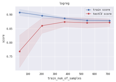
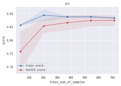
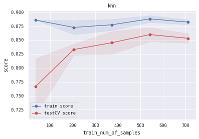
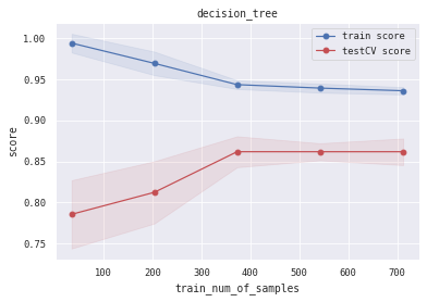
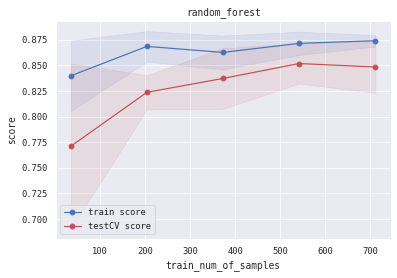
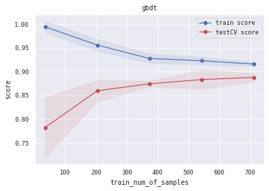
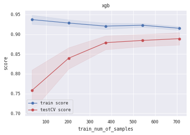
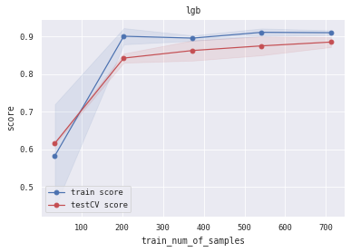
6.5 训练/验证过程可视化 将模型训练过程的学习曲线打印出来,看下是否存在过拟合/欠拟合情况
1 2 3 4 5 6 7 8 9 10 11 12 13 14 15 16 17 18 19 20 21 22 23 24 25 26 27 28 29 30 31 32 33 34 35 36 37 38 39 40 def plot_learning_curve (clf, title, X, y, ylim=None , cv=None , n_jobs=3 , train_sizes=np.linspace(.05 , 1. , 5 ):1 )1 )1 )1 )111 )if ylim is not None :u"train_num_of_samples" )u"score" )0.1 , color="b" )0.1 , color="r" )'o-' , color="b" , label=u"train score" )'o-' , color="r" , label=u"testCV score" )"best" )1 ] + train_scores_std[-1 ]) + (test_scores_mean[-1 ] - test_scores_std[-1 ])) / 2 1 ] + train_scores_std[-1 ]) - (test_scores_mean[-1 ] - test_scores_std[-1 ])return midpoint, diff'logreg' , 'svc' , 'knn' , 'decision_tree' , 'random_forest' , 'gbdt' , 'xgb' , 'lgb' ]0 ], alg_list[0 ], X_all, Y_all)1 ], alg_list[1 ], X_all, Y_all)2 ], alg_list[2 ], X_all, Y_all)3 ], alg_list[3 ], X_all, Y_all)4 ], alg_list[4 ], X_all, Y_all)5 ], alg_list[5 ], X_all, Y_all)6 ], alg_list[6 ], X_all, Y_all)7 ], alg_list[7 ], X_all, Y_all)
(0.8944812361959231, 0.04456088047192275)
1 2 3 4 5 6 7 8 9 10 11 12 13 14 15 16 17 18 19 20 21 22 23 24 25 26 27 28 29 30 from sklearn.metrics import precision_scoreclass Bagging (object def __init__ (self,estimators ):for i in estimators:0 ])1 ])def fit (self, train_x, train_y ):for i in self.estimators:for i in self.estimators]).Tdef predict (self,x ):for i in self.estimators]).Treturn self.clf.predict(x)def score (self,x,y ):return s
6.6 模型集成与验证(Bagging) 选择训练结果最好的四个基学习器进行集成(Bagging)
1 2 3 4 5 6 7 8 9 10 'xgb' ,xgb),('logreg' ,logreg),('gbdt' ,gbdt), ("lgb" , lgb)])from sklearn.metrics import precision_score
X_all,Y_all中按照4:1的比例划分训练数据和测试数据,简化起见没有划分验证集(validation data)用于参数调优,使用训练数据训练我们的集成模型。在划分的测试集上进行预测,并计算模型准确率(Accuracy)。
1 2 3 4 5 6 7 8 9 score = 0 for i in range (0 ,20 ):0.20 round (bag.score(X_cv, Y_cv) * 100 , 2 )20
88.43750000000001
七、进行预测 1 2 3 4 5 6 7 8 int )"PassengerId" : test_df["PassengerId" ],"Survived" : Y_testr'predictedData.csv' , index=False )
八、评价与总结
数据集选择了经典的kaggle数据竞赛中的Titanic数据集。对于我这样的数据科学、机器学习初学者来说,在该数据集基础上可以找到大量来自大神的实现参考,利于快速上手入门;
没有花时间在’’炼丹’’上,只是使用sklearn.model_selection模块中的网格参数搜索函数GridSearchCV进行了较为简单的参数选择。不过我们还是在训练集和测试集都表现出了较高的精度 ,同时没有明显的过拟合或者欠拟合现象。
起初只是想学习并做一个使用GBDT算法的小项目(基于XGboost),但是发现了大神使用集成的方法进行过相关的实现,所以虚心进行了学习 (•ิ_•ิ)
本人知识,经验十分有限,如果有处理不当或者错误的地方还请谅解。
完结撒花 。:.゚ヽ(。◕‿◕。)ノ゚.:。+゚